The FlowTracker's Dependence Graph

This work presents an algorithm to build the SSA Graph with data and control dependences. We guarantee that our technique creates at most O(V ) control dependence edges, where V is the number of variables in the input program. As we point out, the Ferrante's approach can create a graph with O(V2) control dependence edges. One of the benefits of our algorithm is its simplicity: we can describe it in less than 40 lines of executable SML code. And the beauty of our approach is that live range splitting lets us extend the reach of this very algorithm to any kind of program.

We have implemented our technique in the LLVM compiler, and have built the SSA graph of the programs present in the SPEC CPU 2006 benchmark suite. To demonstrate the applicability of our ideas, we use them to implement the flow sensitive type system proposed by Hunt and Sands. We then use this type system to discover four different kinds of information-flow related vulnerabilities. The first, which we call the address disclosure problem, allows an adversary to circumvent Address Space Layout Randomization, a protection commonly used in modern operating systems. We are the first group to provide a tool to point out this kind of vulnerability. The second vulnerability that we analyze is the ever-present buffer overflow. We use our dependence graphs to mark which memory loads can be influenced by an adversary who controls the program’s input channels. We also use our dependence graphs to track integer overflow related vulnerabilities that can compromise memory allocation. Finally, we have a tool to detect side channels vulnerabilities in crypto codes, which can be accessed at this link. Even though the first two analyses are forward, and the third is backward, we can implement them in the same way, as slices of the SSA graph.

SML Prototye of our Algorithm

  /*If pw == in returns 1, else returns 0 */
  datatype Instruction =
    UNY of string * string
  | BIN of string * string * string
  | PHI of string * string * string
  | RET;

datatype DomTree =
    BRANCH of Instruction list * string * DomTree list * DomTree
  | JUMP of Instruction list * DomTree list

fun link [] _ = []
  | link _ "" = []
  | link ((UNY (a, _)) :: insts) label = (label, a) :: link insts label
  | link ((BIN (a, _, _)) :: insts) label = (label, a) :: link insts label
  | link ((PHI (a, _, _)) :: insts) label = (label, a) :: link insts label

fun visit (JUMP (instructions, nil)) pred =
          link instructions pred
  | visit (JUMP (instructions, [child])) pred =
          link instructions pred @ visit child pred
  | visit (BRANCH (instructions, new_pred, children, pdom)) pred =
          let
            fun visit_every nil = nil
              | visit_every (child::rest) =
                if child = pdom
                then visit child pred @ visit_every rest
                else visit child new_pred @ visit_every rest
          in
            link instructions pred @ visit_every children
          end

(* Dominance Tree *)
val t19_19 = JUMP ([UNY ("max0", "len")], []);
val t20_22 = JUMP ([PHI ("max1", "max0", "max"), BIN ("sum1", "sum",
      "len")], []);
val t17_18 = BRANCH ([BIN ("b2", "len", "max")], "b2", [t19_19,
t20_22], t20_22);
val t15_16 = JUMP ([BIN ("len1", "len", "1"), BIN ("p1", "p", "1")], []);
val t10_14 = BRANCH ([PHI ("p", "p0", "p1"), PHI("len", "len0",
      "len1"), BIN ("t", "p", "0"), BIN ("b1", "t", "EOS")], "b1",
    [t15_16, t17_18], t17_18);
val t8_9 = JUMP ([BIN ("p0", "v", "i"), UNY ("len0", "0")], [t10_14]);
val t23_24 = JUMP ([BIN ("maxr", "0", "max"), UNY ("sumr", "sum")], []);
val t3_7 = BRANCH ([PHI ("i", "i0", "i1"), PHI ("max", "max0",
      "max1"), PHI ("sum", "sum0", "sum1"), BIN ("b0", "i", "N")], "b0",
    [t8_9, t23_24], t23_24);
val t0_2 = JUMP ([UNY ("i0", "0"), UNY ("sum0", "0"), UNY ("max0",
      "0")], [t3_7]);

(* Driver *)
val ans = visit t0_2 "";
     

Below we can see an example where Ferrante's approach generates a high number of control edges. This is a classical Control Flow Graph named Ladder Graph. For this case, Ferrante's work give us a quadradic number of control edges according ladder size grows.

Worst case to Ferrante's approach - Ladder Graph

int main(int argc, char** argv) {
  int v = argc;
L0:
  v = argc * 2;
  if (argc == 0 ) {
    goto L2;
  } else {
    goto L1;
  }
L1:
  goto L3;
L2:
  v = argc * 4;
  if (argc == 2 ) {
    goto L4;
  } else {
    goto L3;
  }
L3:
  goto L5;
L4:
  v = argc * 6;
  if (argc == 4 ) {
    goto L6;
  } else {
    goto L5;
  }
L5:
  goto L7;
L6:
  v = argc * 8;
  if (argc == 6 ) {
    goto L8;
  } else {
    goto L7;
  }
L7:
  goto L9;
L8:
  goto L9;
L9:
  return v;
}
     

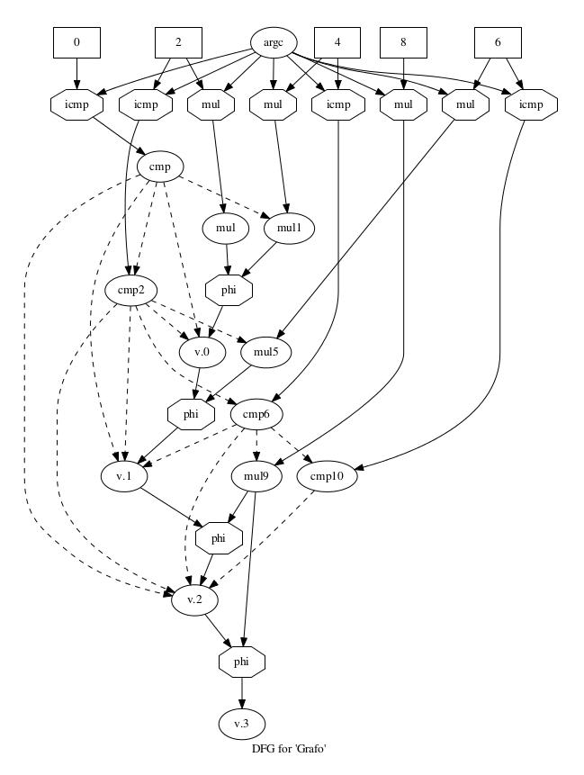
Related to the example above, we can produce two very different dependence graph, which are presented below. On the left side the Ferrante's dependence graph is clearly bigger than (15 control edges) our approach at right side (9 control edges).

Ferrante's Dependence Graph	Flow Tracker Dependence Graph

The Ladder CFG can be produced automatically by the following python script. To execute it, just copy and paste the code in a blanck file and type python file.py ladderSize > file.c.

Python script to generate Ladder CFG

import sys

def genlad(n):
  print "int main(int argc, char** argv) {"
  print "  int v = argc;"

  for BB in range(0, n):
    print "L" + str(2*BB) + ":"
    print "  v = argc * " + str(2*BB + 2) + ";"
    print "  if (argc == " + str(2*BB) + " ) {"
    print "    goto L" + str(2 * (BB+1)) + ";"
    print "  } else {"
    print "    goto L" + str(2 * (BB+1) - 1) + ";"
    print "  }"
    print "L" + str(2*BB + 1) + ":"
    print "  goto L" + str(2 * BB + 3) + ";"

  print "L" + str(2 * n) + ":"
  print "  goto L" + str(2 * n + 1) + ";"
  print "L" + str(2 * n + 1) + ":"
  print "  return v;"
  print "}"

if len(sys.argv) < 2:
  print "Syntax: " + sys.argv[0] + " [num of steps in ladder]"
else:
  numSteps = int(sys.argv[1])
  genlad(numSteps)
    

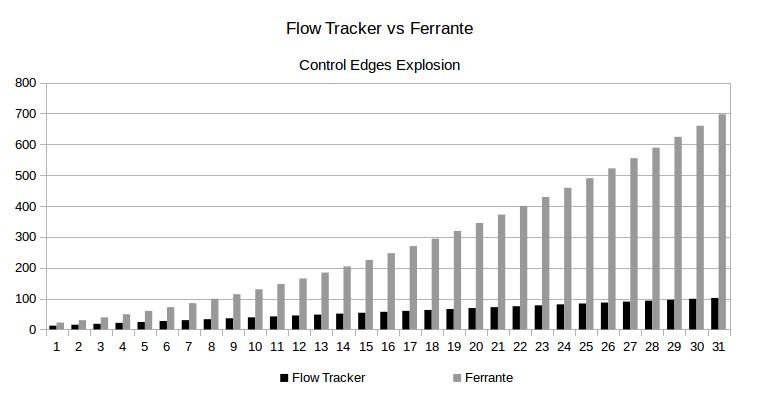
Below we can see a chart showing how the number of control edges grows according Ladder Size is increased.

If you are interesting in our work, you can access the FlowTracker main page and download the passes to LLVM compiler or download our Virtual Box virtual machine which has Flow Tracker deployed. We also provide a web page to detect side channels vulnerabilides in C/C++ codes, which uses the Flow Tracker.

Contact